Ceci est une ancienne révision du document !
ATIAM Music machine learning
This section summarizes the courses in machine learning applied to music computing given along the ATIAM Masters at IRCAM.
Courses
Supervised and AI
- Introduction to artificial intelligence
- Properties of machine learning
- Neural networks
From supervised to unsupervised
- Support Vector Machines
- Properties of kernels
- Clustering algorithms
Probabilistic Graphical Models
- Probability and Bayesian inference
- Undirected graphical models
- Expectation maximization
Advanced Models
- Gaussian mixture models
- Hidden Markov models
- Deep learning
- Applications
Tutorials
The present tutorials covers coding exercices designed to implement the core notions seen in the machine learning lessons. Most techniques can be applied to any type of data from which sets of features can be computed. The exercices here target these techniques specifically applied to musical or audio data.
Part 1. Introduction
In the introduction, we will cover basic Music Information Retrieval (MIR) interactions, in which we process a dataset of sound files and try to observe the properties of their various temporal and spectral features.
1.0 - Reference code
Get the baseline code from this link
1.1 - Datasets
In order to do so, we will work with several datasets that should be downloaded on your local computer first from this link
- Classification - MuscleFish dataset
- Music-speech - MIREX Recognition set
- Source separation - SMC Mirum dataset
- Speech recognition - CMU Arctic dataset
For the first parts of the tutorial, we will mostly use the classification dataset only. In order to facilitate the interactions, we provide the function importDataset that allows to import different audio datasets
function dataStruct = importDataset(classPath, type)
% classPath  : Path to the dataset (string)
% type       : Type of dataset (string: 'classify', 'plain', 'metadata')

% Returns the dataStruct structure with
dataStruct.filenames  % Cell containing the list of audio files
dataStruct.classes    % Vector of indexes assigning each file to a class
dataStruct.classNames % Cell of class names
Exercice to perform
1.2 - Preprocessing
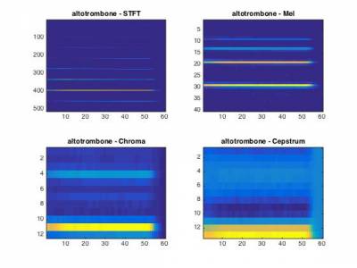
We will rely on a set of spectral transforms that allow to obtain a more descriptive view over the audio information. As most of these is out of the scope of the machine learning course, we redirect you to a signal processing course proposed by Julius O. Smith.
The following functions to compute various types of transforms are given as part of the basic package, in the 0b_Preprocessing folder
stft.m- Short-term Fourier transformfft2barkmx.m- Bark scale transformfft2melmx.m- Mel scale transformfft2chromamx- Chromas vectorspec2cep.m- Cepstrum transformcqt.m- Constant-Q transform
In order to perform the various computations, we provide the following function, which performs the different transforms on a complete dataset.
function dataStruct = computeTransforms(dataStruct)
% dataStruct   : Dataset structure with filenames

% Returns the dataStruct structure with
dataStruct.spectrumPower     % Power spectrum (STFT)
dataStruct.spectrumBark      % Spectrum in Bark scale
dataStruct.spectrumMel       % Spectrum in Mel scale
dataStruct.spectrumChroma    % Chroma vectors
dataStruct.spectrumCepstrum  % Cepstrum
dataStruct.spectrumConstantQ % Constant-Q transform
Exercice to perform

1.3 - Features
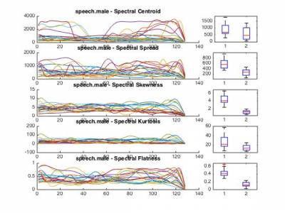
As you might have noted from the previous exercice, most spectral transforms have a very high dimensionality, and might not be suited to exhibit the relevant structure of different classes. To that end, we provide a set of functions for computing the following features in the 0c_Features folder
featureSpectralCentroid.m- Spectral centroidfeatureSpectralCrest.m- Spectral crestfeatureSpectralDecrease.m- Spectral decreasefeatureSpectralFlatness.m- Spectral flatnessfeatureSpectralKurtosis.m- Spectral kurtosisfeatureSpectralRolloff.m- Spectral rollofffeatureSpectralSkewness.m- Spectral skewnessfeatureSpectralSlope.m- Spectral slopefeatureSpectralSpread.m- Spectral spreadfeatureMFCC.m- Mel-Frequency Cepstral Coefficients (MFCC)
Once again, we provide a function to perform the computation of different features on a complete set. Note that for each feature, we compute the temporal evolution in a vector along with the mean and standard deviation of each feature. We only detail the resulting data structure for a single feature.
function dataStruct = computeFeatures(dataStruct)
% dataStruct   : Dataset structure with filenames

% Returns the dataStruct structure with
dataStruct.SpectralCentroid     % Temporal value of a feature
dataStruct.SpectralCentroidMean % Mean value of that feature
dataStruct.SpectralCentroidStd  % Standard deviation
Exercice to perform

Part 2. Nearest neighbors
In this tutorial, we will cover the simplest querying and classification algorithms derived from the k-Nearest Neighbor method. The idea is to find the closest neighbor to a point by assessing its multi-dimensional distance to the rest of the dataset.
INSERT MATH HERE
By looking at the previously given definitions, start by thinking about the following questions.
Questions
2.2 - Querying
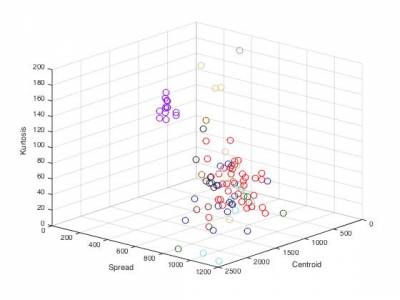
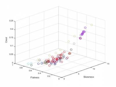
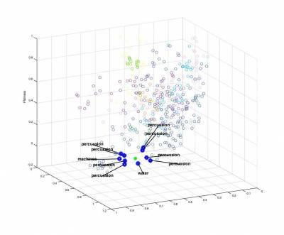
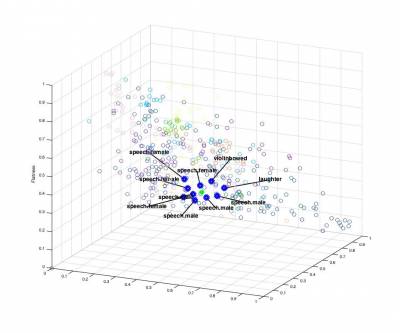
In a first step, we can use the nearest-neighbor method to devise a very simple querying system. This type of method is typically used in many systems such as Query By Humming (QBH) softwares (similar to Shazam). As previously, we provide a baseline code in the main script. This allows to create a n x f distance matrix dataMatrix corresponding to the features of the n elements of the datasets. We selected here only the SpectralCentroidMean, SpectralFlatnessMean and SpectralSkewnessMean features.
Exercice to perform
usedFeatureslist
2.2 - Classification
For the second part of this tutorial, we will rely on the same technique (computing the distance of a selected point to the rest of the dataset) in a classification framework. The overarching idea behind kNN classification is that elements from a same class should have similar properties in the feature space. Hence, the closest feature to those of an element should be from elements of its right class. These types of approaches are usually termed as distance-based classification methods.
function [probas, winnerClass] = knnClassify(dataStruct, testSample, k, normalize, useL1dist);
% This function is used for classifying an unknown sample using the kNN
% algorithm, in its multi-class form.
%
% Arguments :
% - dataStruct  : the data structure
% - testSample  : the input sample id to be classified
% - k           : the k (number of neighbors) parameter
% - normalize   : use class priors to weight results
% - useL1dist   : use L1 instead of L2 distance
% Returns :
% - probas      : an array that contains the classification probabilities for each class
% - winnerClass : the label of the winner class
Exercice to perform
knnClassifycode to perform the k-NN classification function
2.3 - Evaluation
When proposing new algorithms for machine learning problems, the fundamental aspects of corresponding research lies in correctly evaluating their performances. Depending on the application, method proposed, dataset and even the nature of corresponding data, a plethora of evaluation measures can be used. We highly recommend the following articles for those interested in future work around machine learning, so that you develop your critical mind and do not limit yourself to narrow evaluations (by relying on statistical tests) and also that you avoid cherry picking
- Demšar, J. (2006). Statistical comparisons of classifiers over multiple data sets. The Journal of Machine Learning Research, 7, 1-30. [ PDF Link ]
- Sturm, B. L. (2013). Classification accuracy is not enough. Journal of Intelligent Information Systems, 41(3), 371-406. [ PDF Link ]
- Keogh, E., & Kasetty, S. (2003). On the need for time series data mining benchmarks: a survey and empirical demonstration. Data Mining and knowledge discovery, 7(4), 349-371. [ PDF Link ]
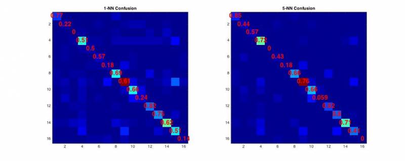
However, for the scope of this tutorial, we will stick to the typical measures that are minimally required to evaluate your classifier. Overall, the most important aspects of evaluation lies in different ways of comparing the real labels (ground truth) to the assigned labels (picked by the classifier).
- The confusion matrix is computed simply by counting the occurences in which a particular instance of a real label (row) is classified to an assigned label (column). This code is already provided in the starter code, and all the following measures can be derived directly from it.
- The overall accuracy is computed as the ratio of correctly classified examples divided by the complete number of examples.
- The (per-class) precision defines the ratio of examples correctly assigned to a class divided by the number of instances assigned to that class by the classifier.
- The (per-class) recall defines the ratio of examples correctly assigned to a class divided by the number of instances really belonging to that class.
- The F1 measure is defined as the ratio between the geometric and harmonic means between the precision and recall measures.
You can implement these measures by simply completing the starter code. If you have doubts about the implementation of these measures, you can check the corresponding Wikipedia article
Part 3. Neural networks
In this tutorial, we will cover a more advanced classification algorithm through the use of neural networks. The tutorial starts by performing a simple single neuron discrimination of two random distributions. Then, we will study the typical XOR problem by using a more advanced 2-layer perceptron. Finally, we generalize the use of neural networks in order to perform classification on our set of audio files.
To simplify your work, we provide the following set of functions that you should find in the 2_Neural_Networks folder
plot3view.m- Allows to plot a 3-dimensional view of data pointsplotBoundary.m- Plots the decision boundary of a single neuron with 2-dimensional inputsplotBoundarySurface.m- Plots the decision surface of a single neuron with 3-dimensional inputsplotBpBoundary.m- Plots multiple decision boundaries for a set of hidden unitsplotBpPats.m- Plots input patterns for back-propagationplotPats.m- Plots input patterns for single neuron problemsplotPats3D.m- Plots 3-dimensional input patterns for single neuron problemsxorAns.dat- Class values for the XOR problemxorPats.dat- Point values for the XOR problem
3.1 - Single neuron discrimination
For the first parts of the tutorial, we will perform the simplest classification model possible in a neural network setting, a single neuron. We briefly recall here that
Therefore, a single neuron can only perform a linear discrimination of the space. We will start by training a single neuron to learn how to perform this discrimination with a linear problem (so that it can solve it). To produce such classes of problems, we provide a script that draw a set of random 2-dimensional points, then choose a random line in this space that will act as the linear frontier between 2 classes (hence defining a linear 2-class problem). The variables that will be used by your code are the following.
patterns      % 2 x n matrix of random points
desired       % classes of the patterns
inputs        % 3 x n final matrix of inputs (accounting for bias)
weights       % 3 x 1 vector of neuron weights
Exercice to perform


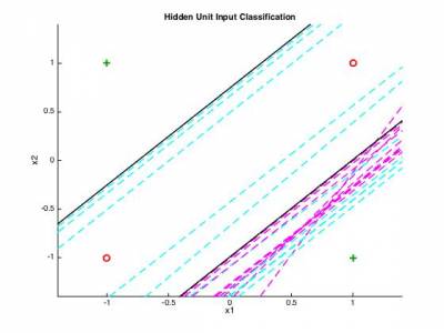
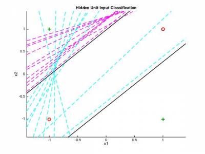
3.2 - 2-layer classification on the XOR problem
In most cases, classification problems are far from being linear. Therefore, we need more advanced methods to be able to compute non-linear class boundaries. The advantage of neural networks is that the same principle can be applied in a layer-wise fashion. This allows to further discriminate the space in sub-regions (as seen in the course). We will try to implement the 2-layer perceptron that can provide a solution to the infamous XOR problem. The idea is now to have the output of the first neurons to be connected to a set of other neurons.
We provide the prototypical set of XOR values in the xorPat.mat along with their class values in xorAns.mat The variables that will be used by your code are the following.
patterns          % 2 x n matrix of random points
desired           % classes of the patterns
inputs1           % 3 x n final matrix of inputs (accounting for bias)
nHiddens          % Number of hidden units
learnRate         % Learning rate parameter
momentum          % Momentum parameter
weights1          % 1st layer weights
weights2          % 2nd layer weights
TSS_Limit         % Sum-squared error limit
Exercice to perform
3.3 - 3-layer generalization to audio classification
We now return to our original classification problem and will try to perform neural network learning on a set of audio files. The data structure will be the same as the one used for parts 1 and 2. As discussed during the courses, even though a 2-layer neural network can provide non-linear boundaries, it can not perform "holes" inside those regions. In order to obtain an improved classification, we will now rely on a 3-layer neural network. The modification to the code of section 3.2 should be minimal, as the back-propagation will be similar for the new layer as one of the two others.
Exercice to perform
Part 4. Support Vector Machines
In this tutorial, we will cover a more advanced classification algorithm through the use of Support Vector Machines (SVMs). The goal is to gain an intuition of how SVMs works and how to use Gaussian kernel with SVMs to find out the decision boundary. The implementation proposed here follows the Sequential Minimal Optimization (SMO) algorithm for training support vector machines. You can find the full details on the mathematics involved in the following paper link.
Once again, to simplify your work, we provide the following set of functions that you should find in the 3_Support_Vector_Machines folder
example1.mat- Example data for a quasi-linear problemexample2.mat- Example data for a non-linear but well-defined problemexample3.mat- Example data for a slightly non-linear problem with outliersplotData.m- Allows to plot the set of data pointsvisualizeBoundary.m- Plots a non-linear decision boundary from a SVM modelvisualizeBoundary.m- Plots a linear decision boundary
4.1 - Linear classification
For the first part of this tutorial, we will compute the main iterations of the algorithm (minimization of the objective function), while relying on a linear kernel. This implies that we will only be able to perform linear discrimination. However, remember that the SVM will provide an optimal and (gloriously) convex answer to this problem.
function pred = svmPredict(model, X)
% Returns a vector of predictions using a trained SVM model (svmTrain).
% X       : m x n matrix where each example is a row.
% model   : svm model returned from svmTrain.
% pred    : m x 1 column vector of class predictions ({0, 1} values).
function [model] = svmTrain(X, Y, C, kernelFunction, tol, maxIter)
% Trains an SVM classifier using a simplified SMO algorithm.
% X       : m x n matrix of m training examples (with n-dimensional features).
% Y       : column vector of class identifiers
% C       : standard SVM regularization parameter
% tol     : tolerance value used for determining equality of floating point numbers.
% maxIter : number of iterations over the dataset before the algorithm stops.
Exercice to perform
svmTraincode to perform the training of a SVM with linear kernel.svmTrainfunction on theexample1.mat(linear) dataset, you should obtain the result displayed below.


4.2 - Gaussian kernel
Exercice to perform
svmTraincode to be able to rely on a Gaussian (RBF) kernel instead of a linear one.svmTrainfunction on theexample2.mat(non-linear) dataset, you should obtain the result displayed below.


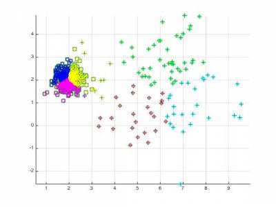
Part 5. Clustering
In this part, we will use the principles of clustering to perform spectral grouping. The idea is to automatically discover the structure inside a spectrogram by using the simplest algorithm of clustering (k-Means algorithm). Hence, even though the results might be slightly drafty, it can give you a good sense of how to automatically uncover structure in an unsupervised way.
5.1 K-Means algorithms
First to perform the implementation of the K-Means algorithm, the following exercises will rely on a first synthetic dataset (linearly separated Gaussian distributions generated similarly to the SVM exercises). Hence, we will create a data set from two Gaussian distributions in a two-dimensional space.
Then, to evaluate the limitations of the K-Means algorithm, we will generate a dataset of two circle distributions. We briefly recall here that the most basic way to perform data clustering is to first start with a random guess of the cluster centroids and then alternate between assigning the data points to different clusters and then updating the centroids of corresponding clusters.
Exercice to perform
kmeansppfunction to implement the clustering algorithm.

5.4 Descriptors and grouping
We will now try to rely on the clustering functions that we just devised to perform an unsupervised grouping of a dataset of audio files. We already provided the code to perform this task, however the tuning is still to be made.
Exercice to perform
kmeansppfunction works on spectral features with 2 clusters.
5.2 - Spectral Grouping
In this section, we will rely on the previously implemented kMeans algorithm to perform a spectral clustering and observe the obtained clusterings. By completing the code yourself, try to perform a binarization followed by a clustering of spectrograms in order to group spectral components together.
Part 6. Gaussian Mixture Models
Part 7. Deep Learning
In this exercise, we will use the self-taught learning paradigm with a sparse autoencoder and (optionnaly in the supplementary exercice) softmax classifier to build both a classifier for spectral windows, but also an unsupervised audition system.
First, you will train your sparse autoencoder on an unlabeled training dataset of audio data (in this case, you can use all the datasets from the tutorials, and even add your own audio files), which will be represented as a set of concatenated spectral windows (to keep the temporal information. This should produce features that are similar to the current theory of Spectro-Temporal Receptive Fields (SRTF), which models neurons in the primary auditory cortex (A1).
Then, we will extract these learned features from the labeled dataset of audio files. These features will then be used as inputs to a softmax classifier. Concretely, for each example in the the labeled training dataset, we forward propagate the example to obtain the activation of the hidden units. This transformed representation is used as the new feature representation with which to train the softmax classifier.
8.1 - Sparse Auto-Encoders (SAE)
We will rely on the set of spectral transforms described in the first exercice.
In the starting code, we provide the basic functions to perform
???.m- ??????.m- ???
In order to perform the various computations, we will use the minFunc package and develop the following function
function dataStruct = computeTransforms(dataStruct)
% dataStruct   : Dataset structure with filenames

% Returns the dataStruct structure with
dataStruct.???     % ???
dataStruct.???     % ???
dataStruct.???     % ???
We will use the unlabeled data (any audio files) to train a sparse autoencoder. However, we first need to prepare an input set, so that the given data is formatted to a common size (slices of audio input). In the following problem, you will implement the sparse autoencoder algorithm, and show how it discovers an optimal representation for spectral windows.
Specifically, in this exercise you will implement a sparse autoencoder, trained with 4 consecutive spectral distributions (FFT, Mel, Bark or Cepstrum) using the L-BFGS optimization algorithm (this algorithm is provided in the minFunc subdirectory, which is a 3rd party CCA software implementing L-BFGS).
Generating inputs
The first step is to generate a training set. To get a single training example x, we need to compute the spectral transform from a sound and then subsample a set of a given number of consecutive spectral frames. This will allow the network to learn from the complete spectro-temporal information. However, the sampled parts will need to be converted into vectors.
Exercice to perform
svmTraincode to perform a cross-validation .svmTrainfunction on theexample3.matdataset, you should obtain the result displayed below.
Sparse autoencoder objective
As seen in course, the learning of an autoencoder is based on a cost function that tries to reconstruct the input from a combination of hidden units. The sparsity aspects allow to force the network to make this reconstruction from fewer data. To do so, we need to both define the cost function Jsparse(W,b) and the corresponding derivatives of Jsparse with respect to the different parameters.
We will use the sigmoid function for the activation function, f(z) = \frac{1}1-e-z} and complete the code in sparseAutoencoderCost.m.
The sparse autoencoder is parameterized by matrices W^{(1)} \in \Re^{s_1\times s_2}, W^{(2)} \in \Re^{s_2\times s_3} vectors b^{(1)} \in \Re^{s_2}, b^{(2)} \in \Re^{s_3}. However, for subsequent notational convenience, we will "unroll" all of these parameters into a very long parameter vector θ with s1s2 + s2s3 + s2 + s3 elements. The code for converting between the (W(1),W(2),b(1),b(2)) and the θ parameterization is already provided in the starter code.
Implementational tip: The objective Jsparse(W,b) contains 3 terms, corresponding to the squared error term, the weight decay term, and the sparsity penalty. You're welcome to implement this however you want, but for ease of debugging, you might implement the cost function and derivative computation (backpropagation) only for the squared error term first and then add both the weight decay and the sparsity term to the objective and derivative function
In order to test the validity of your implementation, you can use the method of gradient checking, which allows you to verify that your numerically evaluated gradient is very close to the true (analytically computed) gradient.
Implementational tip: If you are debugging your code, performing gradient checking on smaller models and smaller training sets (e.g., using only 10 training examples and 1-2 hidden units) may speed things up.
Exercice to perform
svmTraincode to perform a cross-validation .svmTrainfunction on theexample3.matdataset, you should obtain the result displayed below.Do not forget to vectorize your code for speed
8.2 - Training the SAE and visualizing
Once you have coded and verified your objective and derivatives, you can train the parameters of the model and use it to extract features from the spectral windows. Equiped with the code that computes Jsparse and its derivatives, we're ready to minimize Jsparse with respect to its parameters, and thereby train our sparse autoencoder.
We will use the L-BFGS algorithm. This is provided to you in a function called minFunc (code provided by Mark Schmidt) included in the starter code. (For the purpose of this assignment, you only need to call minFunc with the default parameters. You do not need to know how L-BFGS works). We have already provided code in train.m (Step 4) to call minFunc. The minFunc code assumes that the parameters to be optimized are a long parameter vector; so we will use the "θ" parameterization rather than the "(W(1),W(2),b(1),b(2))" parameterization when passing our parameters to it.
Train a sparse autoencoder with 4xN input units, 200 hidden units, and 4xN output units. In our starter code, we have provided a function for initializing the parameters. We initialize the biases b^{(l)}_i to zero, and the weights W^{(l)}_{ij} to random numbers drawn uniformly from the interval \left[-\sqrt{\frac{6}{n_{\rm in}+n_{\rm out}+1}},\sqrt{\frac{6}{n_{\rm in}+n_{\rm out}+1}}\,\right], where nin is the fan-in (the number of inputs feeding into a node) and nout is the fan-in (the number of units that a node feeds into).
Visualization After training the autoencoder, use display_network.m to visualize the learned weights. (See train.m, Step 5.).
Exercice to perform
svmTraincode to perform a cross-validation .svmTrainfunction on theexample3.matdataset, you should obtain the result displayed below.Do not forget to vectorize your code for speed
8.3 - Logistic regression model
In softmaxCost.m, implement code to compute the softmax cost function J(θ). Remember to include the weight decay term in the cost as well. Your code should also compute the appropriate gradients, as well as the predictions for the input data (which will be used in the cross-validation step later).
Implementation Tip: Computing the ground truth matrix - In your code, you may need to compute the ground truth matrix M, such that M(r, c) is 1 if y© = r and 0 otherwise. This can be done quickly, without a loop, using the MATLAB functions sparse and full. Specifically, the command M = sparse(r, c, v) creates a sparse matrix such that M(r(i), c(i)) = v(i) for all i. That is, the vectors r and c give the position of the elements whose values we wish to set, and v the corresponding values of the elements. Running full on a sparse matrix gives a "full" representation of the matrix for use (meaning that Matlab will no longer try to represent it as a sparse matrix in memory). The code for using sparse and full to compute the ground truth matrix has already been included in softmaxCost.m.
Implementation tip: Preventing overflows
In the softmax regression, we compute the unbounded hypothesis of the input belonging to each class, which can lead to overflow. However, given the definition of the logistic function, the overall (relative) probabilities remain equivalent if we substract the same quantity from each of the \theta_j^T x^{(i)}. Hence, to prevent overflow, we shall simply subtract some large constant value from each of the \theta_j^T x^{(i)} terms before computing the exponential.
Implementation tip: Computing the predictions
You may also find bsxfun useful in computing your predictions. If you have a matrix M containing the e^{\theta_j^T x^{(i)}} terms, such that M(r, c) contains the e^{\theta_r^T x^{©}} term, you can use the following code to compute the hypothesis (by dividing all elements in each column by their column sum)
% M is the matrix as described in the text
M = bsxfun(@rdivide, M, sum(M))
Gradient checking
Once you have written the softmax cost function, you should check your gradients numerically. In general, whenever implementing any learning algorithm, you should always check your gradients numerically before proceeding to train the model.
Learning parameters
Now that you've verified that your gradients are correct, you can train your softmax model using the function softmaxTrain in softmaxTrain.m. softmaxTrain which uses the L-BFGS algorithm, in the function minFunc.
Exercice to perform
svmTraincode to perform a cross-validation .svmTrainfunction on theexample3.matdataset, you should obtain the result displayed below.Do not forget to vectorize your code for speed
8.4 - Classifying the test set
Finally, complete the code to make predictions on the test set (testFeatures) and see how your learned features perform! If you've done all the steps correctly, you should get an accuracy of about 98% percent. As a comparison, when raw pixels are used (instead of the learned features), we obtained a test accuracy of only around 96% (for the same train and test sets).
Exercices
This
References
- Linear algebra revision slides from Andrew Ng
- Probability revision slides from Andrew Ng
- Statistics course notes from William Faris
- Sampling pages 20 to 31 from Iain Murray
- Matrix calculus in the Matrix Cookbook